R Markdown for Novices: All you need to know to get started
I write this blogpost for someone, who has never worked with R Markdown. After you read this post, you will
understand why R Markdown may be useful for your daily work as a student, researcher, analyst or data scientist.
understand the basic structure of an R Markdown document and how you can get startet.
I strongly encourage everybody working with R to use R Markdown. I promise, it will make your life so much easier. Here are some examples when R Markdown can be very useful:
Results sharing: You just did a great analysis and want to share your results with your team. Then you start copy pasting your Output into Excel, Word or PowerPoint. Don't do that! It takes so much time and you might forget to copy paste the most curret version of a plot or an analysis. R Markdown can automatically convert your results to many formats such as html, word and pdf. No more copy pasting necessary! This will not only save you lot's of time, it is also less error prone: With R Markdown, everything is up to date automatically!
Data exploration You are looking at various summary statistics and plots to understand your data. Without R Markdown, you might scroll through your console and use the back and forward button in the R Studio Viewer. This is cumbersome! You can use R Markdown like a Notebook and see multiple output tables and plots without having to use the RStudio Viewer back buttons. At the same time, you can see the code, that produced the plot. Which brings me to my next point:
Replicable Analyses: In general, all your results should be repoducible. If you just save a plot or a result, do you know exaclty which steps you needed? If you're a really organized person, this might be possible with naming conventions. But again, R Markdown can make your life so much easier: You can save your results (e.g. a plot or a table) and the code that created it, in one file.
Automated reports: With R Markdown, you can automate analyses that need to be consistent and in the same format every time.
So how does it work?
In an R Markdown File (.Rmd) you can combine R code chunks and text (which is written in a Markdown language. More in a second!). Your R code will be excecuted and your results will be displayed. Everything is "knitted" together to a Markdown format, which can be converted into almost any format through Pandoc. The outputfile may contain your code, formated text (executed Markdown) and the R output (tables, plots, numbers...). This may sound complicated. But all you have to do is write this file, choose your output format and press the "Knit" button in R studio.
Sounds magical? Let's create your first R Markdown file in R Studio. I encourage you to use R Studio, because it provides a lot of awesome features, which simplify working with R Markdown.
Go to File --> New File --> R Markdown.
Choose a Title. It does not matter and can be changed easily afterwards
Choose your desired output (Word, Pdf...) format. Let's choose html as a start!
(Maybe do you need to install additional packages, R Markdown will tell you which)
There is your first R Markdown file. It already contains a little code. Let's talk about the structure of an R Markdown document.
.Rmd File Strucutre
There are 3 different kind of code.
- YAML Header
- Markdown
- R Code Chunks
If you press the "Knit" button, you see, that this runs perfectly and creates an output file. You just successfully compiled your first .Rmd file! A window with your output file should open up. Let's look at the 3 different kinds of code in your .Rmd example file.
YAML Header
The header is on top of every .Rmd file. The code is enclosed with 3 dashes. Your Header contains meta data about your .Rmd file, such as the author, date and output format. You can add additional stuff such as gloabal variables. But don't worry about your header too much for now. Let it just be there.
---
title: "My first R Markdown document"
author: "Heike W"
date: '2018-11-05'
output: html_document
---
Markdown (Text)
Markdown is a simple textformatting language. Similar to HTML or Latex, you write plain text. Punctuation characters indicate the formating. For example a # header1 indicates a header on the top level. You can make you text italic by enclosing it in 2 asterisk (*italic*). If you have never worked with HTML, Latex or Markdown before, this may appear strange to you: Your text appears to have no format. You cannot see how your formatting looks like until you compile the document. You have to click on the "Knit" button to compile your R Markdown. Then you will see the formating of your output file.The good thing is that you can be sure, that a header level 1 is a header level 1 and all header level 1 will look the same in the final document. Here is an overview of the most common formating:
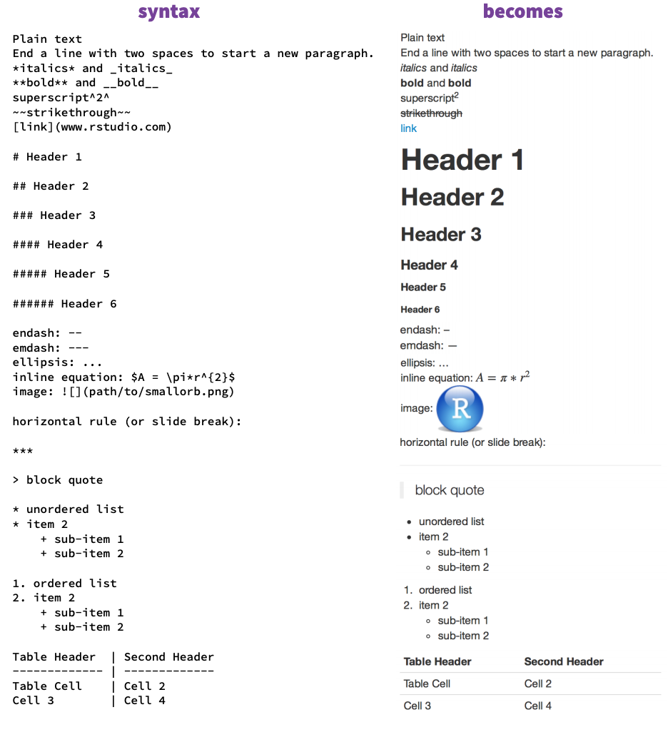
Source RMarkdown Cheat Sheet
R Code Chunks
Just write your R code and wrap it around 3 apostrophies followed by {r}. This tells R Markdown that you want to write R code (You could also insert for example python {python}, bash {bash} or sql {sql}). Insert as many code chunks as you want. Instead of typing 3 apostrophies and the curly braces everytime, you can simply press command-option-I on the Mac and Ctrl-Alt-I on Windows to create a new code chunk. Per default, R will execute this code chunk and display the code and the results in the output file when you "knit" your .Rmd file.
```{r headCars}
summary(cars)
```
You have previously executed the example code by clicking on the "Knit" button in R Studio. This opens a new session and runs the entire .Rmd file. This means you're starting with a new clean environment. You can also run single R code chunks separately. Click on the little green triange in the right corner of your code chunk and only this chunk will run. You can see, that the results are shown directly below your code.
You can give names to your code chunks within the curly braces of your R code chunks. I named our first code chunk "headCars". In addition, you can pass options. Options tell R what it should do with this code chunk. For example, for not displaying any R code in the output file pass echo = FALSE:
```{r headCars, echo = FALSE}
summary(cars)
```
Or you can tell R not to run a code chunk by setting eval = FALSE.
```{r headCars, eval = FALSE}
summary(cars)
```
You can use as many options as neccessary. The order of options does not matter, but you have to separate them with a comma.
```{r headCars, echo = TRUE, eval = FALSE}
summary(cars)
```
Here is a brief overview of the options, I use the most.
| How should the output look like? | How to change the parameter | Default option? |
|---|---|---|
| include code | echo = TRUE | yes |
| automatically format code | tidy = TRUE | no |
| do not execute code | eval = FALSE | no |
| execute code, but show nothing | include = FALSE | no |
| do not show any warnings | warings = FALSE | no |
| do not show any errors | error = FALSE | no |
You can find a comprehensive overview about code chunk options on Yihui Xie's website
You're wondering whether you have to pass the same options to all your code chunks? You don't. You can determine global options at the beginning of your .Rmd file Here in this example, where I told R Markdown to not print any code.
```{r globaloptions, include=FALSE}
knitr::opts_chunk$set(echo = FALSE)
```
The code chunk options overwrite the global options. So if there is one code chunk, where you want to display code, you can pass the option echo = TRUE to this code chunk and the code will be shown in the output document.
Insert plots & figures
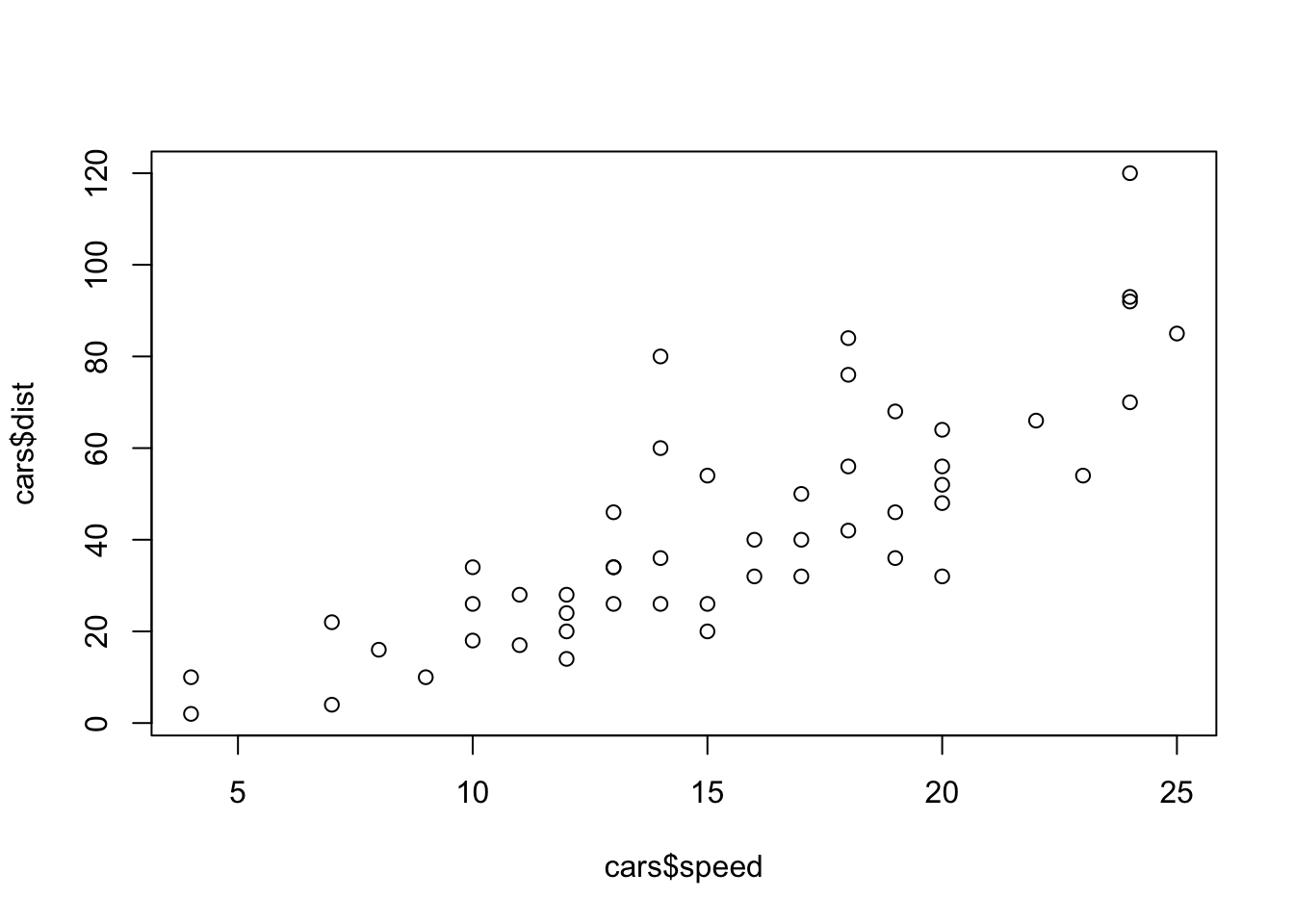
You can easily insert the figures that are created with R code. Just write R code within your code chunks, that creates a plot. R Markdown will insert your plot right after your code.
```{r firstPlot}
plot(cars$speed, cars$dist)
```
As you have done previously, you can use the options of code chunks to alter your output. This works for figures as well. Most figure options start with fig.. For example, you can change the size (fig.height, fig.width (default size = 7 inches)), the alignment (fig.align ("left","right","center")) and the caption (fig.cap) of your plot.
Let's create a wide plot, which with central alignment give it a caption.
r ```{r myWidePlot, fig.height = 4, fig.align = "center", fig.cap = "my wide plot"} plot(cars$speed, cars$dist) ```
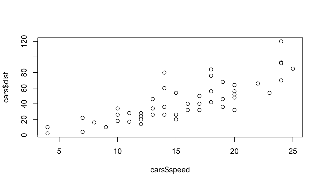
Figure 1: my wide plot
What about local images or GIFS from the internet? You can include them as well. Here is an example. The brackets are optional, if you want a title for the figure. Paste the path to the image into the braces.
My plot caption
Insert Tables
Per default, tables look pretty ugly. R will print the output from the console with leading #.
```{r carsTable}
head(cars)
```
## speed dist
## 1 4 2
## 2 4 10
## 3 7 4
## 4 7 22
## 5 8 16
## 6 9 10You can get rid of the # by using the option comment = FALSE.
```{r carsTable, comment= FALSE}
head(cars)
```
FALSE speed dist
FALSE 1 4 2
FALSE 2 4 10
FALSE 3 7 4
FALSE 4 7 22
FALSE 5 8 16
FALSE 6 9 10Hm, still not very pretty! The kable function from the knitr package provides nicer looking tables.
```{r carsTable, comment= FALSE}
library(knitr)
kable(head(cars))
```
FALSE Warning: package 'knitr' was built under R version 3.5.2| speed | dist |
|---|---|
| 4 | 2 |
| 4 | 10 |
| 7 | 4 |
| 7 | 22 |
| 8 | 16 |
| 9 | 10 |
In the next blogpost, I will go into more detail how you can style your tables.